ToyDL之扩散模型DDPM

背景：某生成任务用到了DDPM，为了更直观理解其前向和反向过程，写个简易的Toy工程

Github地址

扩散模型简介

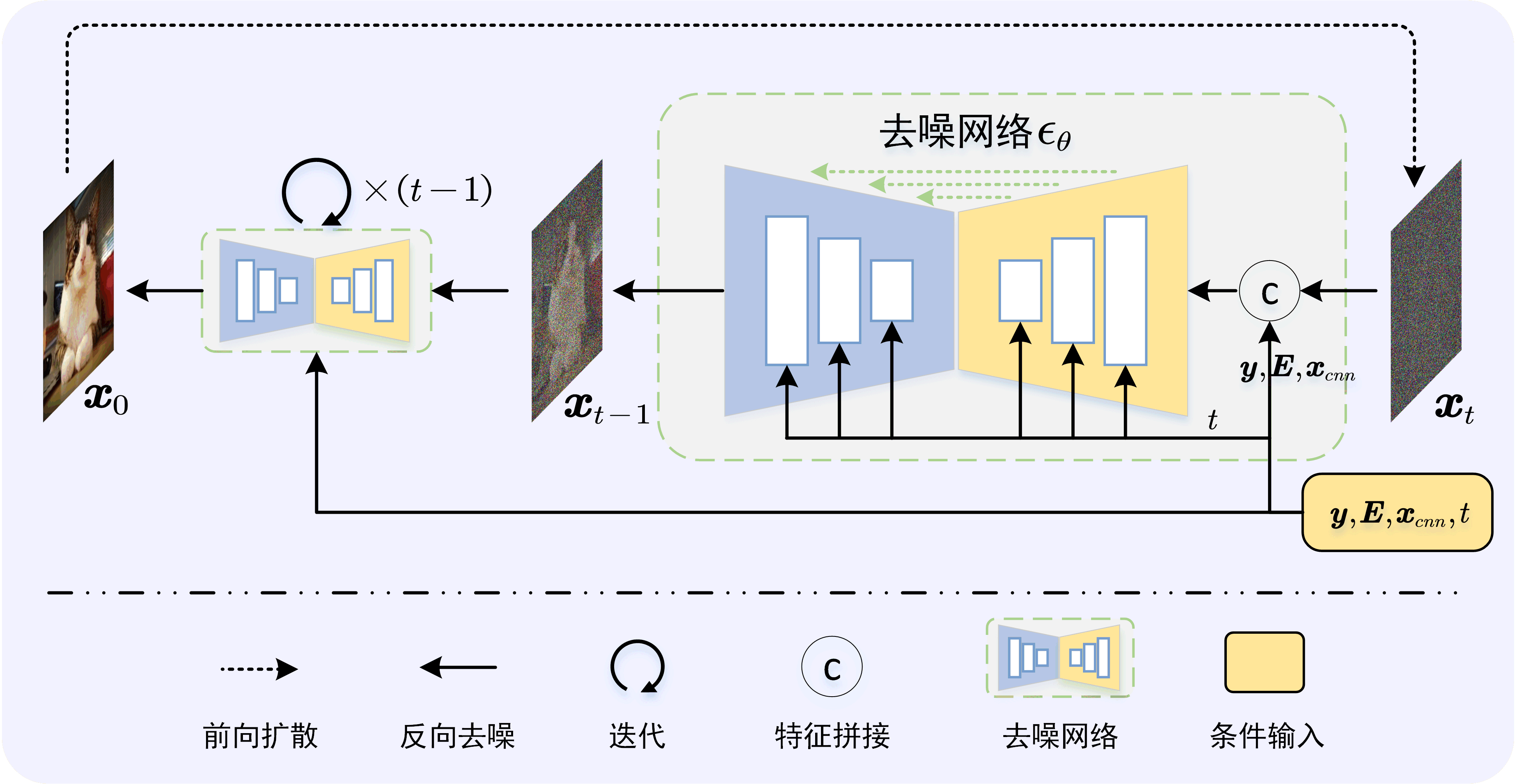
由两条参数化马尔可夫链组成。 前向过程（又称扩散过程）时逐渐向数据中添加噪声，直到数据完全退化为噪声。反向过程则逐步去噪，最终达到数据生成的目的

下两图是毕设中的，条件扩散模型

前向过程

前向为加噪过程，核心公式如下

其中$\bar{\alpha}_t=\textstyle \prod_1^t\alpha_t$

$\alpha_{1:T}\triangleq(\alpha_1,\alpha2,\dots,\alpha_T)$是一组超参数，用以控制每次迭代的噪声方差，并且满足条件$0 < \alpha_t < 1$以确保$t \rightarrow \infty$时方差有界

对应核心代码

sqrt_alphas_cumprod = torch.sqrt(alphas_cumprod)
sqrt_one_minus_alphas_cumprod = torch.sqrt(1 - alphas_cumprod ** 2)

# sample t and noise
t = torch.randint(0, n_steps, (b,)).to(device)
z = torch.randn(b, 1).to(device)

# forward sample xt
xt = sqrt_alphas_cumprod.gather(-1, t).view(-1, 1) * x + sqrt_one_minus_alphas_cumprod.gather(-1, t).view(-1, 1) * z

# denoise
z_pred = denoiser(xt, t)

loss = F.mse_loss(z, z_pred)

反向过程

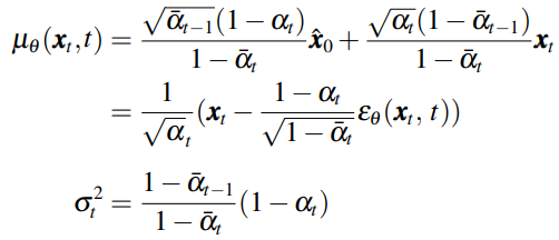
反向采样过程的核心公式如下

对应核心代码

alphas_cumprod_prev = torch.cat([torch.ones(1).to(device), alphas_cumprod[:-1]])
posterior_variance = (1. - alphas) * (1. - alphas_cumprod_prev) / (1. - alphas_cumprod)

def sample_ddpm(x, t):
    t = torch.tensor([t]).to(device)
    at = alphas.gather(-1, t).view(-1, 1)
    st = sqrt_one_minus_alphas_cumprod.gather(-1, t).view(-1, 1)
    mean = torch.sqrt(1.0 / at) * (x - (1.0 - at) * model(x, t.repeat(n_samples)) / st)
    var = posterior_variance.gather(-1, t).view(-1, 1)
    xt_pre = mean + torch.sqrt(var) * torch.randn(n_samples, 1)
    return xt_pre

注意：反向过程需要计算给定$\boldsymbol{x}_0$下的后验分布

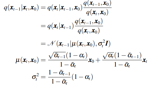
然而反向过程$\boldsymbol{x}_0$未知，DDPM采用的是网络去噪估计$\hat{\boldsymbol{x}}_0=\frac{1}{\sqrt{\bar{\alpha}_t}}(\boldsymbol{x}_t-\sqrt{1-\bar{\alpha}_t}\epsilon_\theta)$，带入上式即可得到反向核心公式

DDIM加速采样

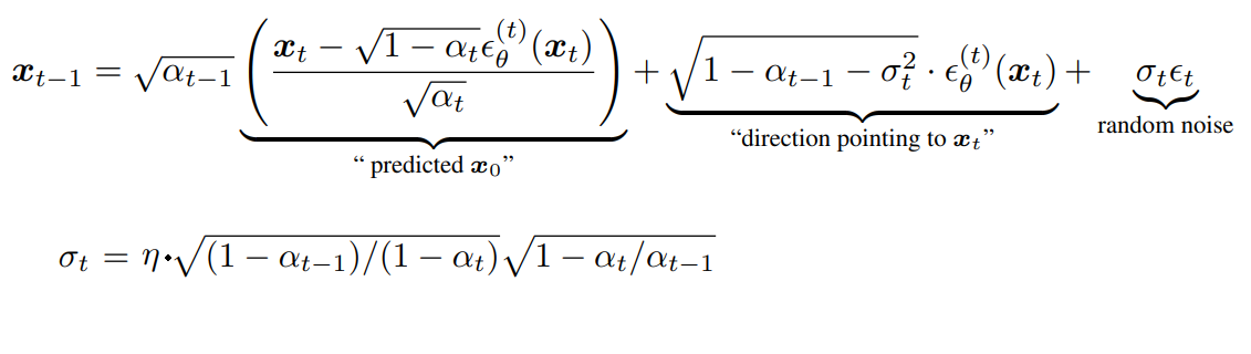
对应核心公式

def sample_ddim(x, t, eta = 1):
    t = torch.tensor([t]).to(device)
    at = alphas_cumprod.gather(-1, t).view(-1, 1)
    at_1 = alphas_cumprod_prev.gather(-1, t).view(-1, 1)
    sigma_t = eta * torch.sqrt((1 - at_1) / (1 - at) * (1 - at / at_1))
    xt_pre = (
        torch.sqrt(at_1 / at) * x 
        + (torch.sqrt(1 - at_1 - sigma_t ** 2) - torch.sqrt(
            (at_1 * (1 - at)) / at)) * model(x, t.repeat(n_samples))
        + sigma_t * torch.randn_like(x)
    )
    return xt_pre

实验对比

以一维数据为例，扩散模型学习给定噪声分布，完成后分别基于DDPM和DDIM进行生成

data = torch.cat([
    torch.randn(30000, 1).to(device) * 0.01 + 0.5,
    torch.randn(40000, 1).to(device) * 0.03 + 0.1,
    torch.randn(30000, 1).to(device) * 0.01 - 0.4,
])

结果如下

可以看出，扩散模型基本可以学出目标数据分布。DDIM可能是由于模型太简单，加速不明显，一般可以10~20倍加速

问答环节

• DDPM为什么慢？
  • 答：因为需要T比较大
• DDPM为什么需要T比较大，能不能缩短步数，或者跳步采样？
  • 答：
• DDIM为什么能加速？
  • 答：

参考

Yuki大佬的扩散模型详解